Real vs Parody Tweet Detection using Bi-Directional LSTM
Analyzing Political Parody in Social Media

This is the second blog of the series Analyzing Political Parody in Social Media paper implementation in the first blog we implemented linear baseline models to classify real vs parody tweets. In this blog, we implement the next level technique with is the Recurrent neural networks, to classify tweets using BiLSTM-Att. Implemented code with dataset uploaded on GitHub.
Bi-LSTM:(Bi-directional long short term memory):
Bidirectional recurrent neural networks(RNN) are really just putting two independent RNNs together. This structure allows the networks to have both backward and forward information about the sequence at every time step
Using bidirectional will run your inputs in two ways, one from past to future and one from future to past, and what differs this approach from unidirectional is that in the LSTM that runs backward you preserve information from the future and using the two hidden states combined you are able in any point in time to preserve information from both past and future.
Data Set
I uploaded a dataset of training and testing related to 1st experiment which is person-based. if you want to get other experiments dataset, you have to email us at talharamzan.tr@gmail.com
Data Pre-Processing
All steps that we carried out in the previous blog for data cleaning and tokenization are the same, you can check the previous blog and code uploaded on GitHub.
BiLSTM-Att
Now lets code
Basic attributes you need to familiar with are
vocab_size: is the number of common words that we want — the maximum number of words that will be included in the word index
oov_token: is the item that will be used to represent words that will not be found in our vocabulary; this is possible when fitting the tokenizer to the testing set. This is represented using the number 1
max_length is the maximum length of each sequence
padding_type: is used to fill zeros either at the beginning or at the end of a sequence
trunction_type: indicates whether to truncate sentences longer than the max_lenth at the beginning or at the end
# Initilize first, i used according to my requirment, you can changevocab_size = 5000
oov_token = "<OOV>"
max_length = 50
padding_type = "post"
trunction_type="post"
Lets Clean data
# Lets clean data
persontrain_df_LSTM.tweet_raw=persontrain_df_LSTM.tweet_raw.apply(clean_dataset)
persontest_df_LSTM.tweet_raw=persontest_df_LSTM.tweet_raw.apply(clean_dataset)
Import Libraries
# Import Librariesfrom tensorflow import keras
from keras.preprocessing.text import Tokenizer
from keras.preprocessing.sequence import pad_sequences
from keras.models import Sequential
from keras.layers import Dense, Embedding, LSTM, Bidirectional
import numpy as np
import pandas as pd
Tokenization
tokenizer = Tokenizer(num_words = vocab_size, oov_token=oov_token)
tokenizer.fit_on_texts(persontrain_df_LSTM.tweet_raw)
Create Sequences
Let’s now convert the sentences into tokenized sequences. This is done using the texts_to_sequences function.
X_train_sequences = tokenizer.texts_to_sequences(persontrain_df_LSTM.tweet_raw)Pad the Sequences
We can clearly see that the sequences are not of the same length, so let’s pad them to make them of similar length — important before we can pass the data to a deep learning model.
X_train_padded = pad_sequences(X_train_sequences,maxlen=max_length, padding=padding_type,
 truncating=trunction_type)
We can now see that there are zeros at the end of the sequences, which makes them all the same length. The padding is taking place at the end of the sequence because we specified the padding type as post.
Now let’s do the same thing to the testing set.
X_test_sequences = tokenizer.texts_to_sequences(persontest_df_LSTM.tweet_raw)
X_test_padded = pad_sequences(X_test_sequences,maxlen=max_length,
                               padding=padding_type, truncating=trunction_type)
Prepare GloVe Embeddings
We’ll use pre-trained embeddings — specifically GloVe embeddings. We start by loading in the GloVe embedding and appending them to a dictionary. You can download it from https://nlp.stanford.edu/projects/glove/
# Loading glove embeddings
embeddings_index = {}
f = open('./glove.6B/glove.6B.200d.txt',
         encoding="utf-8")
for line in f:
    values = line.strip().split(' ')
    word = values[0] # the first entry is the word
    coefs = np.asarray(values[1:], dtype='float32') #100d vectors representing the word
    embeddings_index[word] = coefs
f.close()
Next, we need to create an embedding matrix for each word in the training set. This is done by obtaining the embedding vector for each word from the embedding_index.
embedding_matrix = np.zeros((len(word_index) + 1, 200))
for word, i in word_index.items():
    embedding_vector = embeddings_index.get(word)
    if embedding_vector is not None:
        # words not found in embedding index will be all-zeros.
        embedding_matrix[i] = embedding_vector
Words not found in the embedding index will have a matrix representation with all zeros.
Embedding Layer
- We can now prepare the embedding layer:
- We set
trainableto False because we are using pre-trained word embeddings - We set the
weightsto be the embedding_matrix we created above len(word_index) + 1is the size of the vocabulary. We add one because 0 is never used— it is reserved for paddinginput_lengthis the length of the input sequences
embedding_layer = Embedding(len(word_index) + 1,200,weights=[embedding_matrix],input_length=max_length,trainable=False)Define the Model
from keras.layers import Dropoutembedding_dim = 16
input_length = 100
model = Sequential()
model.add(embedding_layer)
model.add(Dropout(0.2))
model.add(Bidirectional(LSTM(embedding_dim, return_sequences=True)))
model.add(Dropout(0.5))
model.add(Bidirectional(LSTM(embedding_dim)))
model.add(Dense(1, activation='sigmoid'))model.compile(loss='binary_crossentropy',optimizer='adam',metrics=['accuracy'])model.summary()
We use batch size 64 and run this model for 10 epochs
history = model.fit(X_train_padded, persontrain_df.label, epochs=10, batch_size=64,validation_data=(X_test_padded, persontest_df.label))After running we get accuracy on the testing dataset is almost 77%.
# evaluate the model
_, train_acc = model.evaluate(X_train_padded, persontrain_df.label, verbose=0)
_, test_acc = model.evaluate(X_test_padded,  persontest_df.label, verbose=0)
print('Train: %.3f, Test: %.3f' % (train_acc, test_acc))
# plot training history
plt.plot(history.history['loss'], label='train')
plt.plot(history.history['val_loss'], label='test')
plt.legend()
plt.show()#Train: 0.860, Test: 0.768
Then we plot accuracy and loss
# plot the training loss and accuracy
N = 10
plt.style.use("ggplot")
plt.figure()
plt.plot(np.arange(0, N), history.history["loss"], label="train_loss")
plt.plot(np.arange(0, N), history.history["val_loss"], label="val_loss")
plt.plot(np.arange(0, N), history.history["accuracy"], label="train_acc")
plt.plot(np.arange(0, N), history.history["val_accuracy"], label="val_acc")
plt.title("Training Loss and Accuracy on Person wise Dataset")
plt.xlabel("Epoch #")
plt.ylabel("Loss/Accuracy")
plt.legend(loc="best")
plt.savefig("ModelAccuracy(PersonTest-BiLSTM-Att)")
Confusion matrix on test data
y_test_hat = model.predict(X_test_padded, batch_size=64)
y_test_hat = np.round(y_test_hat)conf_m = confusion_matrix(y_test_hat,persontest_df.label)
clas_r = classification_report(y_test_hat,persontest_df.label)# plot confusion matrix as heatmapsns.set(font_scale=1.2)
ax = sns.heatmap(conf_m, annot=True,xticklabels=['Real', 'Parody'], yticklabels=['Real', 'Parody'],
                 cbar=True, cmap='PuBu',linewidths=1, linecolor='black', fmt='.0f')
plt.yticks(rotation=0)
ax.set_ylim([0,2])
plt.xlabel('Predicted labels')
plt.ylabel('True labels')
ax.xaxis.set_ticks_position('top')
plt.title('Confusion matrix')
plt.show()# print classification report
print('Classification report on test data')
print(clas_r)

Conclusion
All code and data set are available on the GitHub repository.
By using LSTM, we achieve almost 78% accuracy. In the next blog, we will use a BERT Transformer model to do this classification.
Paper: A. Maronikolakis, D. Sánchez Villegas, D. Preoţiuc-Pietro, and N. Aletras (2020). Analyzing Political Parody in Social Media. In ACL 2020.
Don’t forget to give us yours 👏 !