Real vs Parody Tweet Detection using Linear Baselines

8 min readJan 22, 2021

Analyzing Political Parody in Social Media

Introduction

Fake news, junk news, or deliberate distributed deception has become a real issue with today’s technologies that allow for anyone to easily upload news and share it widely across social platforms. The Pew Research Center found that 44% of Americans get their news from Facebook. In the wake of the surprise outcome of the 2016 Presidential Election, Facebook and Twitter have come under increased scrutiny to block fake news content from their platform.

I came across the paper, which was very useful and informative to know about NLP techniques to classify which tweets are parody or false and which information is true. In this blog, we implemented the linear baseline models on the dataset which was provided by the authors of the paper. In coming blogs, we also show you how we implemented BiLSTM-Att neural network as well as cutting edge NLP models like the BERT.

In this paper, they performed three experiments on different

Data Set

Collecting Real and Parody Tweets

To develop models that would be able to distinguish between real and parody tweets, we first need to collect a dataset from real and parody accounts respectively.

To collect possible parody accounts, we followed 3 steps:

First, using the Twitter API we query the next terms: parody, #parody, parody account, fake, #fake, fake account, not real.
Then, we manually inspected the tweets from each collected account to make sure that the account constitutes parody.
Next, for each remaining parody account, we found the corresponding real account.

In total, we gathered 103 parody accounts, with 81 of those having a corresponding real account. Around 21% of the accounts are female, while 44% and 26% of all accounts are from the US and UK respectively. From these accounts, we collected all their original tweets (that is, no retweets), balancing the number of real vs. parody tweets within each person to avoid any account overwhelming the dataset.

In total, the data set contains 131,666 tweets, with 65,710 real and 65,956
parody. I uploaded a dataset of training and testing related to 1st experiment which is person-based. if you want to get other experiments dataset, you have to email us at talharamzan.tr@gmail.com

Each row represents one tweet, containing {person, account, tweet_id, tweet_pp, tweet_raw, label} data.

person: Name of the politician (eg. Boris Johnson)
account: Twitter account name (eg. @BorisJohnson)
tweet_id: The id of the given tweet
tweet_pp: The tweet text, pre-processed
tweet_raw: The tweet text, in its original form
label: Whether the tweet is a parody (0) or real (1)

Experiments

We created three data splits for our experiments, and for each data split, we trained and evaluated various machine learning models, including traditional models like logistic regression, to more recent BERT-based approaches that achieve the state of the art in many NLP tasks. BERT is a particular type of transformer network that is pre-trained on language modeling, i.e. given a word in a document, learns to predict its surrounding words.

In this blog, we will share our work using linear baseline models, in the next blogs we will share our implementation of neural network models as well as state of the art NLP techniques like BERT and RoBerta.

The data split and a brief results summary are as follows:

Person Split 😐 In our first experiment, we fed the classifiers tweets from a set of real and parody accounts during training and then tested them to accounts (real and their parody) that they have never seen before.

Gender Split 🙎‍🙎‍♂️ We then split the data by the gender of the politicians. Our aim is to explore whether our classification systems will be able to detect parody from either female or male accounts when they have never trained on them before. That is when testing on female politicians, the train and dev sets are made up of male politicians and vice-versa.

Location Split 🇺🇸🇬🇧🌎 Finally, we split the data according to the location of the politicians (note that we only focus on English speaking countries and accounts that post in English): US, UK, rest of the world (ROW). We perform this experiment to control for the topicality, e.g. politicians from the same country usually discuss similar issues and that may be picked by classifiers making it easy to accurately predict parody.

Problem to be Solved

The problem to be solved by this project is how to identify which tweets are about ‘Real’ and which one’s aren’t. This project will use a data science approach to build a machine learning classifier model to predict which tweets are about ‘real disasters’ and which one’s aren’t.

Project Main Steps:

Data Analysis and Exploration
Data pre-processing
Model Performance Metrics
Vectorization of the pre-processed text
Build a machine learning model
Results
Fine-tune the machine learning model
Challenges and Complications
Conclusion
Improvements

1. Data analysis and exploration

This step is fully implemented in the Jupiter notebook

2. Data Pre-processing

Clean up the Tweets data

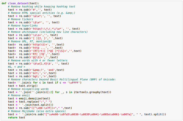
Before we start doing text classification of the tweet we want to clean the tweets as much as possible. We start by removing things like hashtags, hyperlinks, HTML characters, tickers, emojis etc.

For Now, we only use the “Tweet_raw” and “label” columns. Just use the tweets text information as this blog is about text based classification.

Our method, clean_dataset does this.

Tokenization

Tokenization is a process that splits an input text into tokens and the tokens can be a word, sentence, paragraph etc.

The following code will show how tokenization of text works:

# Lets Tokenize the training and the test dataset copies with DLATK, # a Twitter-aware tokenizerfrom happiestfuntokenizing.happiestfuntokenizing import Tokenizer
tokenizer = Tokenizer()
persontrain_df1['tweet_raw'] = persontrain_df1['tweet_raw'].apply(lambda x: tokenizer.tokenize(x))
persontest_df1['tweet_raw'] = persontest_df1['tweet_raw'].apply(lambda x: tokenizer.tokenize(x))

Stopwords Removal

Now, let’s get rid of the stopwords i.e words that occur very frequently and have possible value like a, an, the, are etc.

#Create a funtion to remove stopwords
def remove_stopwords(text):
    
    """
    Input- text=text from which english stopwprds will be removed
    Output- return text without english stopwords 
    
    """
    words = [w for w in text if w not in stopwords.words('english')]
    return wordspersontrain_df1['tweet_raw'] = persontrain_df1['tweet_raw'].apply(lambda x : remove_stopwords(x))
persontest_df1['tweet_raw'] = persontest_df1['tweet_raw'].apply(lambda x : remove_stopwords(x))

3. Vectorization of pre-processed text

Pre-process text needs to be transformed into a vector matrix of numbers before a machine learning model can understand it and learn from it. This can be done by a number of techniques:

1. Bag of Words

The bag of words is a representation of text that describes the occurrence of words within a document. It involves two things:

A vocabulary of known words.
A measure of the presence of known words.

Why is it is called a “bag” of words?
Its called bag of words because any information about the order or structure of words in the document is discarded and the model is only concerned with whether the known words occur in the document, not where they occur in the document.

2. Bag of Words — Countvectorizer Features

Countvectorizer converts a collection of text documents to a matrix of token counts. It is important to note that CountVectorizer comes with a lot of options to automatically do pre processing, tokenization, and stop word removal. However, all the pre processing of the text has already been performed by creating a function. Only a vanilla version of Countvectorizer will be used.

3. TFIDF Features

A problem with the bag of words approach is that highly frequent words start to dominate in the document (e.g. larger score) but may not contain as much “informational content” this will lead to more weight to longer documents than shorter documents.

To avoid that, one approach is to re-scale the frequency of words by how often they appear in all documents so that the scores for frequent words like “the” that are also frequent across all documents are penalized. This approach to scoring is called “Term Frequency-Inverse Document Frequency”, or TF-IDF for short, where:

Term Frequency: is a scoring of the frequency of the word in the current document.

TF = (Number of times term t appears in a document)/(Number of terms in the document)

Inverse Document Frequency: is a scoring of how rare the word is across documents.

IDF = 1+log(N/n), where, N is the number of documents and n is the number of documents a term t has appeared in.

Let’s vectorize train and test data using count vectorizer and TFIDF:

# Vectorize the text using CountVectorizer
count_vectorizer = CountVectorizer(ngram_range=(1,2))
persontrain_cv = count_vectorizer.fit_transform(persontrain_df1['tweet_raw'])
persontest_cv = count_vectorizer.transform(persontest_df1["tweet_raw"])# Vectorize the text using TFIDF
tfidf = TfidfVectorizer(min_df=2, max_df=0.5, ngram_range=(1, 3))
persontrain_tf = tfidf.fit_transform(persontrain_df1['tweet_raw'])
persontest_tf = tfidf.transform(persontest_df1["tweet_raw"])

Build a Text Classification Machine Learning model

LR-BOW (Linear Regression — Bag of Words)

#Define a function to fit and predict on training and test data sets
def fit_and_predict(model,X_train,y_train,X_test,y_test):
    
    '''Input- model=model to be trained
              X_train, y_train= traing data set
              X_test,  y_test = testing data set
       Output- Print accuracy of model for training and test data sets   
    '''
    
    # Fitting a simple Logistic Regression on Counts
    clf = model
    clf.fit(X_train, y_train)
    predictions=clf.predict(X_test)
    conf_m=confusion_matrix(y_test,predictions)
    print(classification_report(y_test,predictions))
    print('-'*50)
    print("{}" .format(model))
    print('-'*50)
    print('Accuracy of classifier on training set:{}%'.format(round(clf.score(X_train, y_train)*100)))
    print('-'*50)
    print('Accuracy of classifier on test set:{}%' .format(round(accuracy_score(y_test,predictions)*100)))
    print('-'*50)
    
    # plot confusion matrix as heatmap
    sns.set(font_scale=1.2)
    ax = sns.heatmap(conf_m, annot=True,xticklabels=['Real', 'Parody'], yticklabels=['Real', 'Parody'], 
                 cbar=True, cmap='RdBu',linewidths=1, linecolor='black', fmt='.0f')
    plt.yticks(rotation=0)
    ax.set_ylim([0,2])
    plt.xlabel('Predicted labels')
    plt.ylabel('True labels')
    ax.xaxis.set_ticks_position('top') 
    plt.title('Confusion matrix - test data\n(Real, Parody) Tweets')
    plt.show()# Create a list of the regression models to be used
models=[LogisticRegression(C=1.0)]# Loop through the list of models and use 'fit_and_predict()' #function to trian and make predictions
for model in models:
    fit_and_predict(model,persontrain_cv,persontrain_df.label,persontest_cv,persontest_df.label)

#TFIDF
for model in models:
    fit_and_predict(model,persontrain_tf,persontrain_df.label,persontest_tf,persontest_df.label)

LR-BOW+POS (Linear Regression — Bag of Words plus Part of Speech)

Part of Speech Tagging POS

def POS(x):
    return nltk.pos_tag(x)
    
persontrain_df_POS['tweet_raw_POS']=persontrain_df_POS['tweet_raw'].apply(lambda x: POS(x))
persontrain_df_POS['tweet_raw_POS'].head()

This section of code also uploaded on my GitHub repository.

Conclusion:

By using linear baseline models, we achieve almost 78% accuracy. In the next blog, we will show you the neural network implementation to classify real and parody tweets.

Paper: A. Maronikolakis, D. Sánchez Villegas, D. Preoţiuc-Pietro, and N. Aletras (2020). Analyzing Political Parody in Social Media. In ACL 2020.

Don’t forget to give us yours 👏 !