Tweet Sentiment Analysis using Logistic Regression from Scratch
Supervised Learning
In this tutorial, I am using the basic NLP (Natural Language Processing) technique to classify tweets in a binary class of positive tweets and negative tweets. For this purpose, I use a supervised learning model logistic regression.

In this tutorial we’d do something like that building a sentiment classifier from scratch based on logistic regression, and we’ll train it on a corpus of tweets, thus we’ll cover :
Text processing
Features extraction
Sentiment classifier
Training & evaluating the sentiment classifier
Text processing
First, we’ll use Natural Language Toolkit (NLTK), it’s an open-source python library, it has a bunch of functions to process textual data, it contains also a Twitter dataset that we’ll work on :
First, import nltk library with some other important libraries for analysis and then download tweet dataset (Corpus) from nltk library
import nltk                              # Python library for NLP
from nltk.corpus import twitter_samples  # sample Twitter dataset from NLTK
import random                        # pseudo-random numbergenerator# downloads sample twitter dataset. uncomment the line below if running on a local machine.nltk.download('twitter_samples')# select the set of positive and negative tweets
all_positive_tweets=twitter_samples.strings('positive_tweets.json')
all_negative_tweets=twitter_samples.strings('negative_tweets.json')print('Number of positive tweets: ',len(all_positive_tweets))
print('Number of negative tweets: ',len(all_negative_tweets))print('\nThe type of all_positive_tweets is:', type(all_positive_tweets))
print('The type of a tweet entry is:', type(all_negative_tweets[0]))
The python code above allows us to get a list of positive tweets and a list of negative tweets. As we download the tweet data from the standard library so both positive and negative tweets numbers are the same, in our case both positive and negative are 5000 each.
import matplotlib.pyplot as plt          # library for visualization# Declare a figure with a custom size
fig = plt.figure(figsize=(5, 5))# labels for the two classes
labels = 'Positives', 'Negative'# Sizes for each slide
sizes = [len(all_positive_tweets), len(all_negative_tweets)]# Declare pie chart, where the slices will be ordered and plotted counter-clockwise:plt.pie(sizes, labels=labels, autopct='%1.1f%%',shadow=True, startangle=90)# Equal aspect ratio ensures that pie is drawn as a circle.
plt.axis('equal')# Display the chart
plt.show()
The above part of the code uses the matplotlib library to draw a pie chart to see the equal distribution of tweets length.

We can print positive tweets in green color and negative tweets in red color. and you can see any tweet which you want only type index number, below code give you an idea how to do different operations on the dataset
# print positive in greeen
print('\033[92m' + all_positive_tweets[random.randint(0,5000)])# print negative in red
print('\033[91m' + all_negative_tweets[random.randint(0,5000)])# Our selected sample. Complex enough to exemplify each step
tweet = all_positive_tweets[2277]
print(tweet)
After doing all this, our main work begins with how to process text, which we call Text Processing.
Tweet data contain a lot of irrelevant information like hashtags, mentions, stop words, etc. Data cleaning or data preprocessing is a key step in the process of data science in order to prepare data for training a classification algorithm. In the context of NLP, text processing includes :
Tokenization: is the operation of splitting a sentence into a list of words.
Removing stop words: stop words refer to the frequent words occurring in a text without adding semantic value to the text.
Removing punctuation: it refers to the marks like (!”#$%&’()*+,-./:;<=>?@[\]^_`{|}~).
Stemming: is the process of reducing a word to its word stem that affixes to suffixes and prefixes or to the roots of words.
We’ll try to implement those operations to process all the tweets before feeding them into our classifier :
Firstly we have to download stopwords data from the nltk library.
nltk.download('stopwords')  #Import the english stop words list from NLTK
stopwords_english = stopwords.words('english')print('Stop words\n')
print(stopwords_english)print('\nPunctuation\n')
print(string.punctuation)
Now we perform different types of text processing techniques.
import re
import stringfrom nltk.corpus import stopwords
from nltk.stem import PorterStemmer
from nltk.tokenize import TweetTokenizer#we'd like to remove some substrings commonly used on the platform like the hashtag, retweet marks, and hyperlinks.print('\033[92m' + tweet)
print('\033[94m')# remove old style retweet text "RT"
tweet2 = re.sub(r'^RT[\s]+', '', tweet)# remove hyperlinks
tweet2 = re.sub(r'https?:\/\/.*[\r\n]*', '', tweet2)# remove hashtags
# only removing the hash # sign from the word
tweet2 = re.sub(r'#', '', tweet2)print(tweet2)print()
print('\033[92m' + tweet2)
print('\033[94m')# instantiate tokenizer class
tokenizer = TweetTokenizer(preserve_case=False, strip_handles=True,
                               reduce_len=True)# tokenize tweets
tweet_tokens = tokenizer.tokenize(tweet2)print()
print('Tokenized string:')
print(tweet_tokens)print()
print('\033[92m')
print(tweet_tokens)
print('\033[94m')tweets_clean = []for word in tweet_tokens: # Go through every word in your tokens list
    if (word not in stopwords_english and  # remove stopwords
        word not in string.punctuation):  # remove punctuation
        tweets_clean.append(word)print('removed stop words and punctuation:')
print(tweets_clean)print()
print('\033[92m')
print(tweets_clean)
print('\033[94m')# Instantiate stemming class
stemmer = PorterStemmer()# Create an empty list to store the stems
tweets_stem = []for word in tweets_clean:
    stem_word = stemmer.stem(word)  # stemming word
    tweets_stem.append(stem_word)  # append to the listprint('stemmed words:')
print(tweets_stem)
Split training and testing data 80% training and 20% testing
import numpy as np   # Python Library NumPytest_pos = all_positive_tweets[4000:]
train_pos = all_positive_tweets[:4000]
test_neg = all_negative_tweets[4000:]
train_neg = all_negative_tweets[:4000]
train_x = train_pos + train_neg
test_x = test_pos + test_neg
train_y = np.append(np.ones((len(train_pos), 1)), np.zeros((len(train_neg), 1)), axis=0)
test_y = np.append(np.ones((len(test_pos), 1)), np.zeros((len(test_neg), 1)), axis=0)
After doing all the text processing step, we will implement a single function for tweets text processing, so that we pass tweets in the function text_process
def text_process(tweet):
    tweet = re.sub(r'^RT[\s]+', '', tweet)
    tweet = re.sub(r'https?:\/\/.*[\r\n]*', '', tweet)
    tweet = re.sub(r'#', '', tweet)
    tokenizer = TweetTokenizer()
    tweet_tokenized = tokenizer.tokenize(tweet)
    stopwords_english = stopwords.words('english')
    tweet_processsed=[word for word in tweet_tokenized
    if word not  in stopwords_english and word not in
    string.punctuation]
    stemmer = PorterStemmer()
    tweet_after_stem=[]
    for word in tweet_processsed:
        word=stemmer.stem(word)
        tweet_after_stem.append(word)
    return tweet_after_stem
Features extraction
After text processing, it’s time for feature extraction. Actually, computers don’t deal with texts, computers only understand the language of numbers, that’s why we should work on transforming tweets into vectors that can be fed into our logistic regression function. We are working on binary classification which means classifying a tweet either positive or negative. So basically, we’d find some words more occurring in the list of positive tweets like happy, good. In the same way, we’d find some words more frequent than the others in the list of negative tweets.
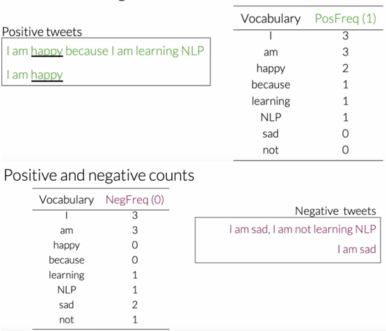
So, in order to implement this, we’ll build the first dictionary containing the frequency of the words in the positive tweets, and the second dictionary will contain the frequency of the words in the negative tweets. Then, well combine the two dictionaries.
pos_words=[]
for tweet in all_positive_tweets:
    tweet=text_process(tweet)

    for word in tweet:

        pos_words.append(word)
freq_pos={}
for word in pos_words:
    if (word,1) not in freq_pos:
        freq_pos[(word,1)]=1
    else:
        freq_pos[(word,1)]=freq_pos[(word,1)]+1
neg_words=[]
for tweet in all_negative_tweets:
    tweet=text_process(tweet)

    for word in tweet:

        neg_words.append(word)
freq_neg={}
for word in neg_words:
    if (word,0) not in freq_neg:
        freq_neg[(word,0)]=1
    else:
        freq_neg[(word,0)]=freq_neg[(word,0)]+1

freqs_dict = dict(freq_pos)
freqs_dict.update(freq_neg)
Each vector is a representation of a tweet. Now, we need to combine those vector in one matrix holding all tweet’s features. As we have 10000 tweets, and each tweet is represented as a vector of 3 dimensions, the shape of our matrix X would be (10000,3) :
def features_extraction(tweet, freqs_dict):
    word_l = text_process(tweet)
    x = np.zeros((1, 3))
    x[0,0] = 1
    for word in word_l:
        try:
            x[0,1] += freqs_dict[(word,1)]
        except:
            x[0,1] += 0
        try:
            x[0,2] += freqs_dict[(word,0.0)]
        except:
            x[0,2] += 0
    assert(x.shape == (1, 3))
    return x
X = np.zeros((len(train_x), 3))

for i in range(len(train_x)):

    X[i, :]= features_extraction(train_x[i], freqs_dict)
Sentiment classifier
To build the sentiment classifier, and instead of using libraries like scikit-learn, we are going to build a logistic regression classifier from scratch :
The logistic or sigmoid function uses the features as input to calculate the probability of a tweet being labeled as positive, if the output is greater or equal to 0.5, we classify the tweet as positive. Otherwise, we classify it as negative.
def sigmoid(x):
    h = 1/(1+np.exp(-x))
    return h

def gradientDescent_algo(x, y, theta, alpha, num_iters):
    m = x.shape[0]
    for i in range(0, num_iters):
        z = np.dot(x,theta)
        h = sigmoid(z)
        J = -1/m*(np.dot(y.T,np.log(h))+np.dot((1-y).T,np.log(1-h)))
        theta = theta-(alpha/m)*np.dot(x.T,h-y)
    J = float(J)
    return J, theta
Training & evaluating the sentiment classifier
After implementing gradient descent, now we’ll move to train in order to calculate the optimal weights theta :
X = np.zeros((len(train_x), 3))
for i in range(len(train_x)):
    X[i, :]= features_extraction(train_x[i], freqs_dict)
Y = train_y
J, theta = gradientDescent_algo(X, Y, np.zeros((3, 1)), 1e-9, 1500)
It’s time for testing our sentiment classifier in order to evaluate how it performs on test_x:
def predict(tweet, freqs_dict, theta):
    x = features_extraction(tweet,freqs_dict)
    y_pred = sigmoid(np.dot(x,theta))
    return y_pred
def test_accuracy(test_x, test_y, freqs_dict, theta):
    y_hat = []
    for tweet in test_x:

        y_pred = predict(tweet, freqs_dict, theta)

        if y_pred > 0.5:

            y_hat.append(1)
        else:

            y_hat.append(0)
    m=len(y_hat)
    y_hat=np.array(y_hat)
    y_hat=y_hat.reshape(m)
    test_y=test_y.reshape(m)

    c=y_hat==test_y
    j=0
    for i in c:
        if i==True:
            j=j+1
    accuracy = j/m
    return accuracy
accuracy = test_accuracy(test_x, test_y, freqs_dict, theta)
We’ve got Model Accuracy: 98.4 %, our model is almost perfect !!
If you are interested in AI, feel free to check out my github: https://github.com/MAbuTalha/Twitter-Sentiment-Analysis. I’ll be putting the source code together with the data there so that you can test it out for yourself. Thank you for reading :)